Hi
I’m trying to put together a script to simplify converting raw data to displacement, velocity, acceleration data. Previously we’ve done this mainly using sac (v101.6a). However using obspy I’m running into trouble reproducing the sac results for displacement and acceleration, whilst output of velocity is within acceptable tolerance. Presumably I’ve missed out on some important point here, so would appreciate any pointers (from what I (miss?)understand by digging through the obspy source obspy make use of evalresp as do sac and although sac stores data as 32-bit most the computations involved mainly uses 64-bit according to the sac manual, in any case the differences I see are to large to be explained by 32-bit vs 64-bit).
Attached here is a raw data (100 Hz sampling rate, 60s instrument) file, data_raw.sac (141.2 KB), as well as a RESP (4.4 KB) file used in the examples below (note that the numbers in the RESP file for the digitizer may look a bit strange, however the file is valid and used both in the sac and obspy instrument de-convolution so should not matter).
The sac results I’m comparing to were produced by use of commands:
displacement
SAC> r data_raw.sac
SAC> rtr
SAC> rmean
SAC> taper type hanning width 0.05
SAC> transfer from evalresp fname RESP freql 0.0117 0.0167 44.0 48.0
SAC> w data_disp_sac.sac
velocity
SAC> r data_raw.sac
SAC> rtr
SAC> rmean
SAC> taper type hanning width 0.05
SAC> transfer from evalresp fname RESP to vel freql 0.0117 0.0167 44.0 48.0
SAC> w data_vel_sac.sac
acceleration
SAC> r data_raw.sac
SAC> rtr
SAC> rmean
SAC> taper type hanning width 0.05
SAC> transfer from evalresp fname RESP to acc freql 0.0117 0.0167 44.0 48.0
SAC> w data_acc_sac.sac
To further aid the comparison of the sac and obspy results I’ve put together a small function to plot the amplitude spectrum (btw. is such a function available in obspy?) in a simple module
ps.py (1.2 KB):
#! /usr/bin/env python3

import numpy as np
import matplotlib.pyplot as plt
def plot_spectrum(st):
   """ plots amplitude spectra """
   axs = []
   ntr = len(st)
   fig = plt.figure(figsize=(14, 10))
   d = []
   for i in range(ntr):
      tr = st[i]
      if i in [2,4]:
         d.append(d[0]-d[i-1])
      else:
         data = tr.data.astype(np.float64)
         fft = np.fft.rfft(data)
         d.append(np.abs(fft))
      fs = [j*tr.stats.sampling_rate/tr.stats.npts for j in range(fft.size)]
      axs.append(fig.add_subplot(ntr,1,i+1))
      axs[-1].semilogy(fs,d[i])
      axs[-1].set_xlim([0,fs[-1]])
      axs[-1].set_ylim([0.01,10**7])
      axs[-1].text(0.02,0.95,tr.id,transform=axs[-1].transAxes,
                  fontdict=dict(fontsize="small", ha='left', va='top'),
                  bbox=dict(boxstyle="round", fc="w", alpha=0.8))
      axs[-1].tick_params(axis="x",which='both',direction="in",top=True,right=True)
      axs[-1].tick_params(axis="y",which='both',direction="in",top=True,right=True)
      if i == (ntr)//2:
         axs[-1].set_ylabel("Amplitude")
      if i < ntr-1:
         axs[-1].xaxis.set_ticklabels([])
   axs[-1].set_xlabel("Frequency (Hz)")

   fig.tight_layout()
   fig.subplots_adjust(hspace=0)
obspy velocity
Conversion to velocity by use of Trace.remove_response(...) works as a charm in terms of comparison to the sac results, difference between sac and obspy results are < 0.1% except at the end points where small differences in tapers used probably is the explanation. For completeness though I add here the script, vel.py (1.3 KB), used.
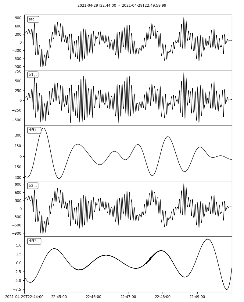
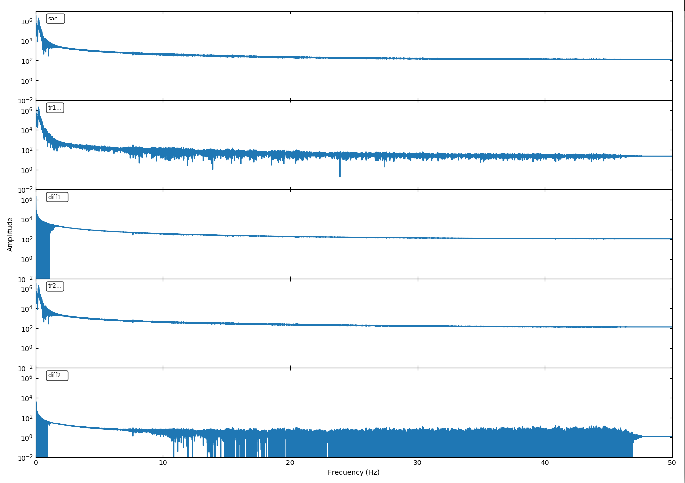
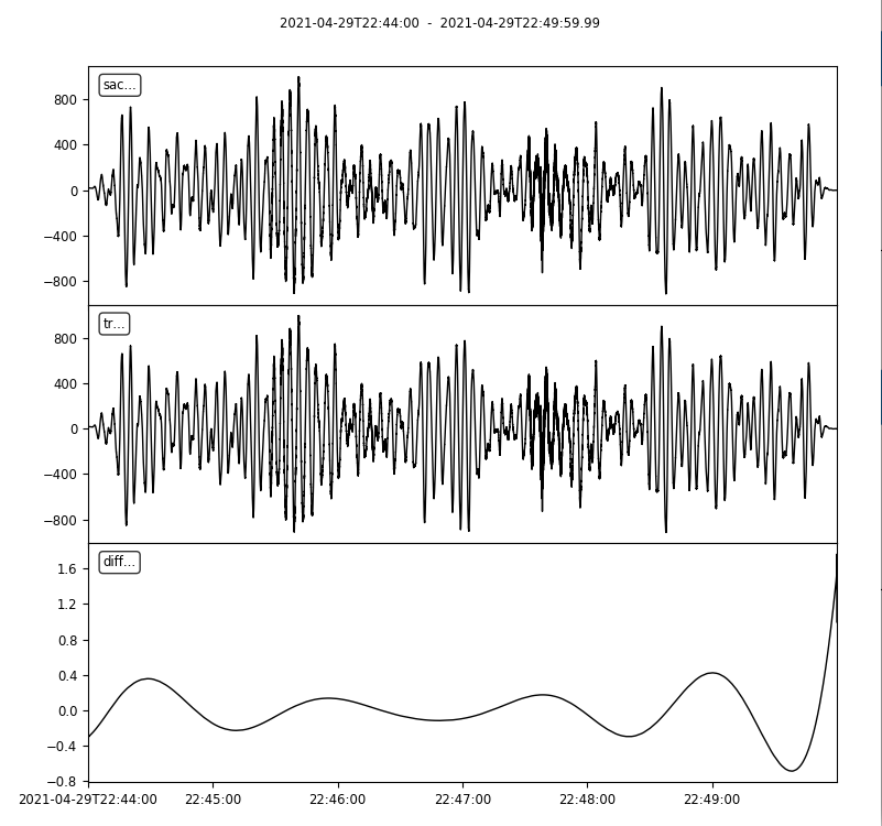
obspy displacements
Conversion to displacement using Trace.remove_response(output="DISP", ...) however yields differences of the order 100% in the time domain and whilst the amplitude spectrum has similar shape there is a significant difference in the amplitude value. For the fun of it I then tried to simply remove the response (counts → velocity) followed by tr.integrate() and strangely enough, suddenly the resulting displacement is within acceptable tolerance (mostly < 1%). The script to reproduce the results, disp.py (1.8 KB), is:
#! /usr/bin/env python3
import obspy
from ps import plot_spectrum

### sac (v101.6a) estimate produced by use of commands:
#  SAC> r data_raw.sac
#  SAC> rtr
#  SAC> rmean
#  SAC> taper type hanning width 0.05
#  SAC> transfer from evalresp fname RESP freql 0.0117 0.0167 44.0 48.0
#  SAC> w data_disp_sac.sac

### Get raw data and respospnse, attach response, remove linear trend, demean and taper
tr = obspy.read("data_raw.sac")[0]
inv = obspy.read_inventory("RESP")
tr.attach_response(inv)
tr.detrend(type="linear")
tr.detrend(type="demean")
tr.taper(type='hann',max_percentage=0.05)

### get two copies of the trace (set meta data to be able to identify in later plot)
tr1 = tr.copy()
tr1.stats.network = "tr1"
tr2 = tr.copy()
tr2.stats.network = "tr2"

### Get displacemnet data as converted by use of SAC (set meta data to be able to identify in later plot)
st = obspy.read("data_disp_sac.sac")
st[0].stats.network = "sac"
st[0].detrend(type="demean")

### Remove response and convert to displacement (nm) in one go

tr.taper(type='hann',max_percentage=0.05)
tr1.remove_response(output="DISP", pre_filt=[0.0117,0.0167,44.0,48.0], zero_mean=True, taper=False)
tr1.data *= 1.e9
tr1.detrend(type="demean")

### Remove response and integrate to displacements (nm) in two steps

tr.taper(type='hann',max_percentage=0.05)
tr2.remove_response(output="VEL", pre_filt=[0.0117,0.0167,44.0,48.0], zero_mean=True, taper=False)
tr2.data *= 1.e9
tr2.integrate()
tr2.detrend(type="demean")

### Compute difference to sac estimate
diff1 = tr1.copy()
diff1.data -= st[0].data
diff1.stats.network = "diff1"
diff2 = tr2.copy()
diff2.data -= st[0].data
diff2.stats.network = "diff2"

### Add obspy estimates and differences to stream object and plot
st += tr1
st += diff1
st += tr2
st += diff2
plot_spectrum(st)
st.plot(automerge=False,equal_scale=False)
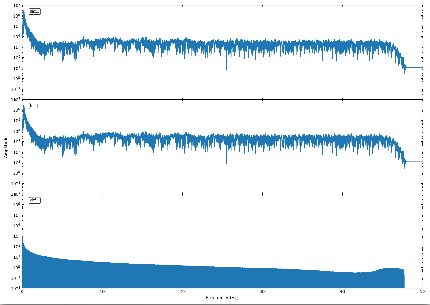
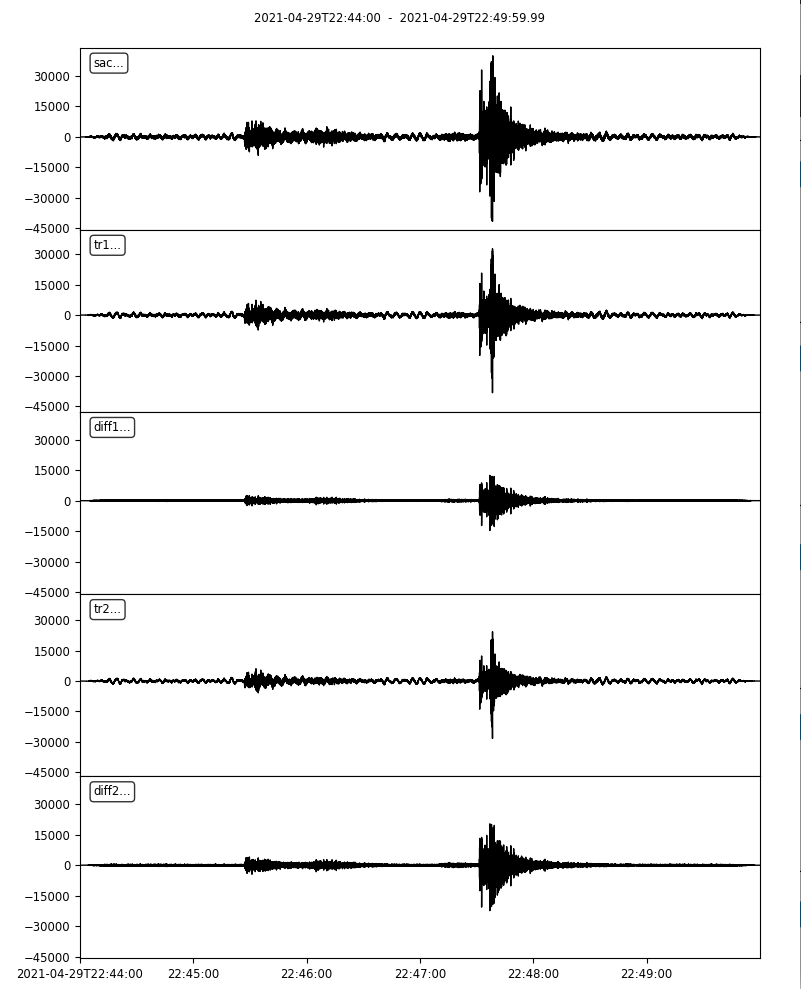
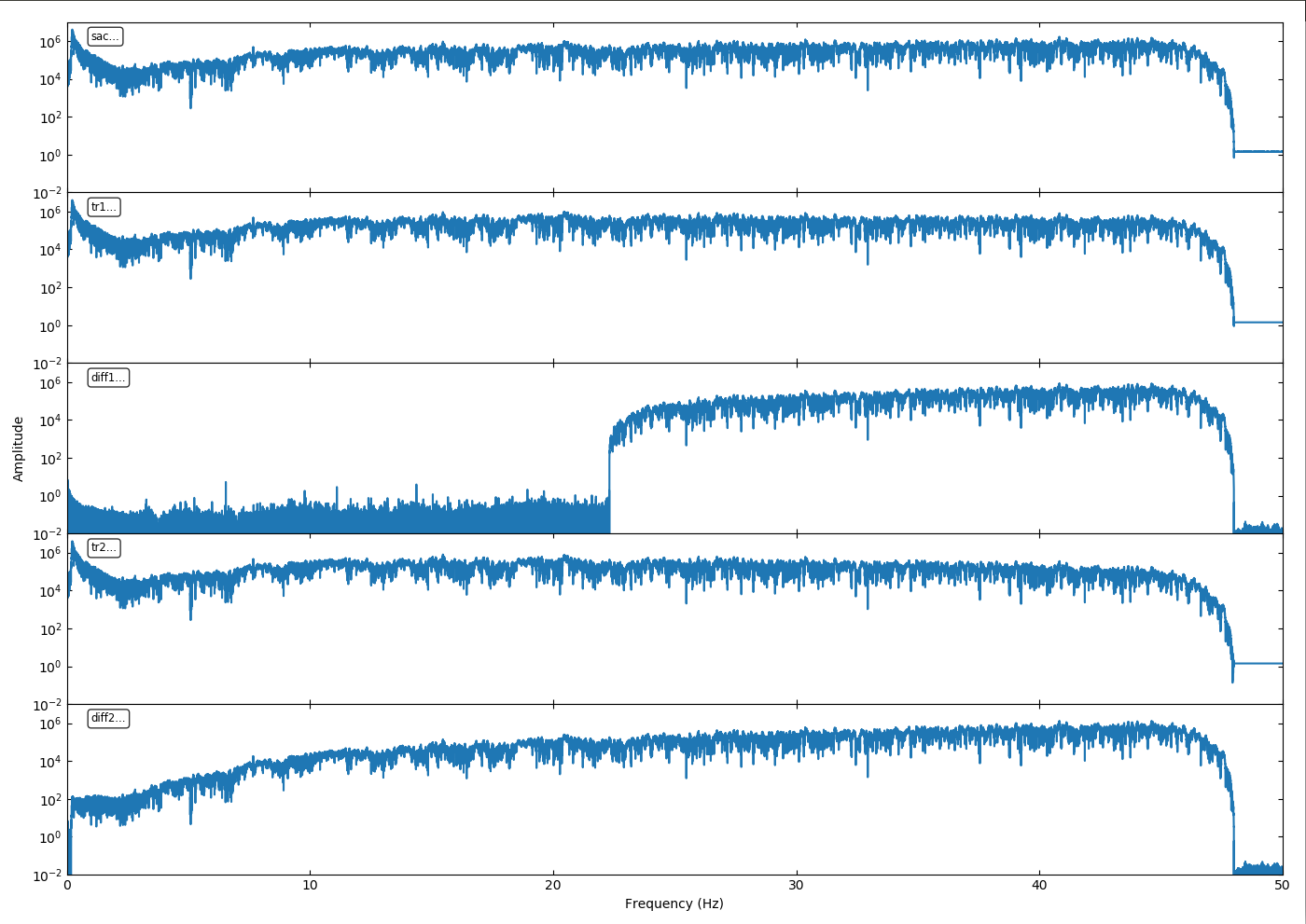
obspy acceleration
Attempting to get to acceleration again there is a significant difference when using Trace.remove_response(output="ACC",...), further inspecting the amplitude spectrum there is a significant increase in the amplitude difference above ~23 Hz. Attempting a similar scheme as used above for the displacements (i.e. only removing response by use of Trace.remove_response(...) followed by Trace.integrate()) unfortunately do not resolve the issue. The script, acc.py (1.9 KB), to reproduce the results is:
#! /usr/bin/env python
import obspy
from ps import plot_spectrum

### sac (v101.6a) estimate produced by use of commands:
#  SAC> r data_raw.sac
#  SAC> rtr
#  SAC> rmean
#  SAC> taper type hanning width 0.05
#  SAC> transfer from evalresp fname RESP to acc freql 0.0117 0.0167 44.0 48.0
#  SAC> w data_acc_sac.sac

### Get raw data and respospnse, attach response, remove linear trend, demean and taper
tr = obspy.read("data_raw.sac")[0]
inv = obspy.read_inventory("RESP")
tr.attach_response(inv)
tr.detrend(type="linear")
tr.detrend(type="demean")
tr.taper(type='hann',max_percentage=0.05)

### get two copies of the trace (set meta data to be able to identify in later plot)
tr1 = tr.copy()
tr1.stats.network = "tr1"
tr2 = tr.copy()
tr2.stats.network = "tr2"

### Get displacemnet data as converted by use of SAC (set meta data to be able to identify in later plot)
st = obspy.read("data_acc_sac.sac")
st[0].stats.network = "sac"
st[0].detrend(type="demean")
#st[0].filter("bandpass",freqmin=0.0167,freqmax=44)

### Remove response and convert to displacement (nm) in one go
tr1.remove_response(output="ACC", pre_filt=[0.0117,0.0167,44.0,48.0], zero_mean=False, taper=False)
tr1.data *= 1.e9
tr1.detrend(type="demean")
#tr1.filter("bandpass",freqmin=0.0167,freqmax=44)

### Remove response and integrate to displacements (nm) in two steps
tr2.remove_response(output="VEL", pre_filt=[0.0117,0.0167,44.0,48.0], zero_mean=False, taper=False)
tr2.data *= 1.e9
tr2.differentiate()
tr2.detrend(type="demean")
#tr2.filter("bandpass",freqmin=0.0167,freqmax=44)

### Compute difference to sac estimate
diff1 = tr1.copy()
diff1.data -= st[0].data
diff1.stats.network = "diff1"
diff2 = tr2.copy()
diff2.data -= st[0].data
diff2.stats.network = "diff2"

### Add obspy estimates and differences to stream object and plot
st += tr1
st += diff1
st += tr2
st += diff2
plot_spectrum(st)
st.plot(automerge=False)
So in summary I can get reasonable results for conversion to velocity and displacement but fail for acceleration (and would preffer to avoid the workaround when converting to displacements) so would appreciate any insight.

