Hello,
I want to plot a spectrogram of the seismic noise for one year or more. I am using mseed files (24 hours). I used the specgram function of matplotlib for processing a 1 hour data window, but I do not know how to concatenate the data in order to have the spectrogram for one year. With my code I just can compute the spectrogram for 1 hour each time.
I know I can plot the spectrogram for large amounts of data with the function ppsd.plot_specgram but I guess this function computes the spectrogram using the McNamara method and I want to apply the Welch method in order to have a spectrogram with more resolution. If someone have a code or know how to fix mine, I will appreciate it, I am new with these topics.
Number of points of windows and overlap for PSD calculation
nfft = 2**15
windlap = 0.5
count = 0 # count the number of traces in the stream
Read frequency response file
inv = read_inventory(“RESP.CW.RCC.00.HHZ”)
filt = [0.009, 0.01, 40, 45]
file_psd = os.listdir() # import the names of all the mseed files
for file in file_psd:
if file.startswith(“CW”):
st = read(file)
name_file = file.split(“.”) #select from the filename the julian day
jday = name_file[6]
st.remove_response(inventory=inv, pre_filt = filt) #remove frequency response
Set the start time Jdays
stime = UTCDateTime("2020-"+jday+"T00:00:00")
etime = stime + 3600
print(stime)
st.trim(stime,etime)
print(st)

hour = range(0, 24) # for processing each 24 hours of the mseed file
for i in hour:
  if len(st) == 0: # in case there is no data in the 1 hour stream
   stime = etime
   etime = stime + 3600
   st = read("CW.RCC.00.HHZ.D.2020."+jday)
   st.trim(stime,etime)
   print("no trace, next")
  else:
    print("trace")

  for index, tr in enumerate(st): # process each trace in stream
    print(tr)
    count = index + 1
    tr.detrend("demean")

    if len(st) > 1 and (count < len(st)):  # in case there is more than 1 trace in the stream
      s, f, t, im = plt.specgram(tr.data, NFFT=nfft,
                    noverlap=int(nfft*windlap), Fs = 1./tr.stats.delta,
                    scale_by_freq=True, detrend="linear", mode="psd")

      plt.colorbar(label='Intensidad (dB)')
      plt.xlabel('s')
      plt.ylabel('Frecuencia (Hz)')
      plt.ylim((0.05, 1.))
      plt.title('Espectrogram')
      plt.show()

      continue

  s, f, t, im = plt.specgram(tr.data, NFFT=nfft,
                    noverlap=int(nfft*windlap), Fs = 1./tr.stats.delta,
                    scale_by_freq=True, detrend="linear", mode="psd")
  stime = etime
  etime = stime + 3600
  st = read("CW.RCC.00.HHZ.D.2020."+jday)
  st.trim(stime,etime)
  plt.colorbar(label='Intensidad (dB)')
  plt.xlabel('s')
  plt.ylabel('Frecuencia (Hz)')
  plt.ylim((0.05, 1.))
  plt.title('Espectrogram')
  plt.show()
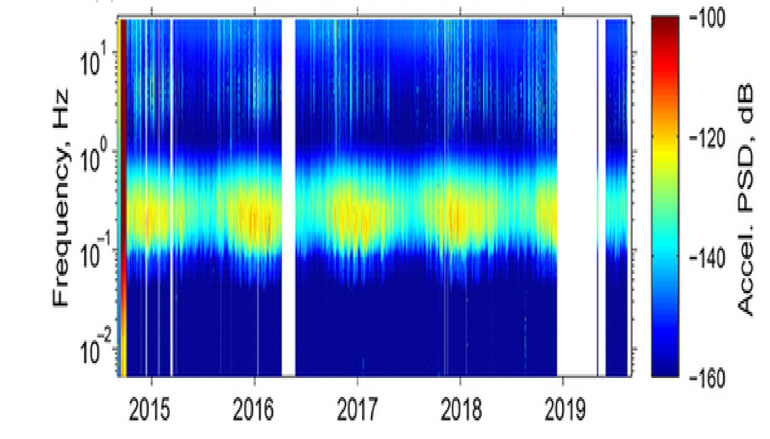
I want to have a plot similar to this one