Hi
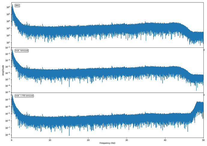
Historically we have not included FIR filter coefficients and decimation stages in our metadata. Discovering however that most(?) other networks do we have started a process towards doing so. However, it seems that this triggers some un-expected behaviour when approaching the Nyquist frequency upon instrument removal. Now while the FIR filter removal should affect the spectral amplitudes close to Nyquist I’m are a bit surprised about the quite high spectral amplitudes resulting from the process (see figure comparing instrument removal including FIR filters or not) thus wondering if this is reasonable or if I’m missing out on something.
To remove the instrument response I’m using the remove_response() method on the Stream object (code example below) and set argument end_stage in the case I wish not to remove the FIR filters.
I’m also wondering a bit about in which order FIR filters and are removed. E.g. when invoking the remove_response() method will it remove the stages in the order they are listed in the metadata (i.e. sensor first, then digitizer, then FIR filters from first to last) or in reverse order (i.e. last FIR filter first and sensor last)? Does it matter which order the stages are removed?
I guess when removing the FIR filters it only makes sense to remove the last FIR filter as previous FIR filter were applied at higher sampling rates and should have minimal to no impact at frequencies up to the Nyquist frequency following the last decimation step, right? However in the response files typically the FIR filters are listed in the order they were applied which means that the last FIR filter is listed last. Upon removal of instrument responses using the remove_response() method one can specify the first and last stage to include but as there may be several FIR filters in the meta data then removing the last FIR filter means that also the previous ones will be removed unless remove response if invoked twice (one time removing the last FIR filter and one time removing the sensor and digitizer response). Now while removing the earlier FIR filters should not affect the data as argued above it does add quite some time to the duration of the operation so when processing a lot of data this can become impractical. Would it perhaps be reasonable to add an argument to the remove_response() method, say use_stage, which takes an iterable where the stages to be removed can be listed (thereby allowing to skip all FIR filters except the last)?
import matplotlib.pyplot as plt
import numpy as np

# Load data and meta data
inv = read_inventory("UP.BLMU.HHZ.dataless")
tr0 = read('UP.BLMU..HHZ.D.20230808T0100-T0130.mseed')[0]

# Demean data and remove linear trend
tr0 = tr0.detrend(type='linear')
tr0 = tr0.detrend(type='demean')
tr0.taper(type='hann',max_percentage=0.005,max_length=2)

# Remove instrument responses only
tr1 = tr0.copy()
tr1.remove_response(inventory=inv, pre_filt=[0.002, 0.008, 49.9, 49.99], end_stage=4)

# Remove instrument responses and FIR filters
tr2 = tr0.copy()
tr2.remove_response(inventory=inv, pre_filt=[0.002, 0.008, 49.9, 49.99])

# Prepare plot
fig = plt.figure(figsize=(14, 10))
axs = []
axs.append(fig.add_subplot(3,1,1,sharex=None))
axs.append(fig.add_subplot(3,1,2,sharex=axs[0]))
axs.append(fig.add_subplot(3,1,3,sharex=axs[1]))

# Make sure data vector to fft is of length equal to 2**n (to speed thing up)
# and set up a frequency vector
n_data = len(tr0.data)
n_use = 2
while n_use*2 <= n_data:
   n_use *= 2
fs = [k*tr0.stats.sampling_rate/n_use for k in range(n_use//2+1)]

# Compute and plot spectral amplitudes
fft0 = np.fft.rfft(tr0.data, n=n_use)
amp0 = np.abs(fft0)
axs[0].semilogy(fs,amp0)
fft1 = np.fft.rfft(tr1.data, n=n_use)
amp1 = np.abs(fft1)
axs[1].semilogy(fs,amp1)
fft2 = np.fft.rfft(tr2.data, n=n_use)
amp2 = np.abs(fft2)
axs[2].semilogy(fs,amp2)

# Add some labels and trim axes
tag = ['ORG', 'Instr. removed', 'Instr. + FIR removed']
for i in range(3):
   axs[i].set_xlim([0, 50])
   axs[i].text(0.02,0.95, tag[i], transform=axs[i].transAxes, fontsize="small", ha='left', va='top', bbox=dict(boxstyle="round", fc="w", alpha=0.8))
axs[1].set_ylabel("Amplitude")
axs[2].set_xlabel("Frequency (Hz)")
fig.tight_layout()
fig.subplots_adjust(hspace=0)

plt.show(block=True)
UP.BLMU..HHZ.D.20230808T0100-T0130.mseed (218.5 KB)
UP.BLMU.HHZ.dataless (24 KB)
The instrument at the site is a nanometrics with a centaur digitizer. The attached dataless file were downloaded directly from the digitizer.
