How to remove polynomial response

Dear All,
I am looking at weather data (LKI, LRO, … channels).
I download the data from FDSN WS.
The attach_response is of course described as a polynomial response.
And unfortunately the “remove_response” does not work for polynomial.
Is there any simple way to remove the polynomial response ?
Is there any plan to modify remove_response to make it working for polynomial resp ?

Thanks,

Mickael.

I see some code for polynomial response in remove_response, so it looks like it should work. Do you have a reproducible, self contained example showing the problem?

Hi Tobias,

Here is the error I am getting :

/Users/langlami/anaconda3/envs/obspy/lib/python3.7/site-packages/obspy/core/inventory/response.py:1193: UserWarning: The unit ‘HPA’ is not known to ObsPy. It will be assumed to be displacement for the calculations. This mostly does the right thing but please proceed with caution.

warnings.warn(msg)

Traceback (most recent call last):

File “./plot_meteo”, line 57, in

st.remove_response()

File “/Users/langlami/anaconda3/envs/obspy/lib/python3.7/site-packages/obspy/core/stream.py”, line 3155, in remove_response

tr.remove_response(*args, **kwargs)

File “/Users/langlami/anaconda3/envs/obspy/lib/python3.7/site-packages/decorator.py”, line 232, in fun

return caller(func, *(extras + args), **kw)

File “/Users/langlami/anaconda3/envs/obspy/lib/python3.7/site-packages/obspy/core/trace.py”, line 273, in _add_processing_info

result = func(*args, **kwargs)

File “/Users/langlami/anaconda3/envs/obspy/lib/python3.7/site-packages/obspy/core/trace.py”, line 2885, in remove_response

output=output, **kwargs)

File “/Users/langlami/anaconda3/envs/obspy/lib/python3.7/site-packages/obspy/core/inventory/response.py”, line 1674, in get_evalresp_response

freqs, output=output, start_stage=start_stage, end_stage=end_stage)

File “/Users/langlami/anaconda3/envs/obspy/lib/python3.7/site-packages/obspy/core/inventory/response.py”, line 1632, in get_evalresp_response_for_frequencies

end_stage=end_stage)

File “/Users/langlami/anaconda3/envs/obspy/lib/python3.7/site-packages/obspy/core/inventory/response.py”, line 1439, in _call_eval_resp_for_frequencies

raise NotImplementedError(msg)

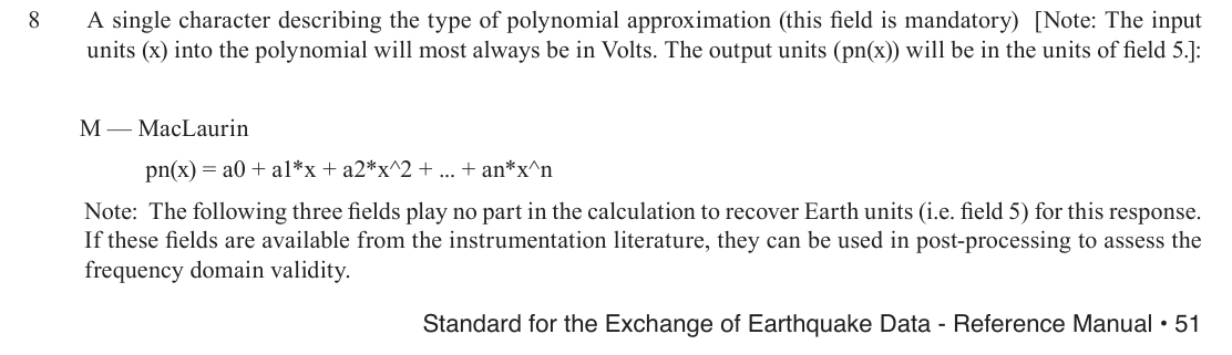
NotImplementedError: PolynomialResponseStage not yet implemented. Please contact the developers.

But I am using obspy 1.2.2 maybe I should migrate to 1.4.0, because as far as I understand this error message polynomial response is not implemented. There is also a warning issu about the unit (here data are pressure in HPA).

Thanks for your comment.

Regards

Mickael.

Yes, please update, first of all things and then let us know how it goes

Hi Tobias,

I have upgraded my obspy to 1.4.0 version. But I have exactly the same error…
Regards

Mickael.

Do you have a self contained minimal example you can share?

Here is the code I am using to test.
First plot without deconvolution, second with, but it fails during the remove_response.

You can try with this command line (assuming the code is named plot_meteo) : ./plot_meteo “2023-11-10T00:00:10” “2023-11-10T12:00:00” “FR.TAMIE.00.L??” --url=“http://ws.resif.fr

-- coding: utf-8 --

“”"
:author:
Mickael Langlais
Usage:
plot_meteo --url=

Example:
plot_meteo “2023-11-10T01:00:00” “2023-11-10T05:00:00” “FR.TAMIE.00.L??” --url=“http://ws.resif.fr

Options:
-h --help Show this screen.
–version Show version.
Start time in obspy.core.UTCDateTime format. Fdsn
mode only.
End time in obspy.core.UTCDateTime format. Fdsn mode
only.
Stream to analyse in seed code separated by dots.
Multiple streams are allowed, separated by comma
–url= Set base url of fdsnws server, fdsn mode only.
[default: http://ws.resif.fr]
“”"
from docopt import docopt
from obspy.clients.fdsn import Client as fClient
from obspy.core import UTCDateTime, Stream, read
from obspy import read_inventory
from obspy.core.inventory.response import Response
from matplotlib import pyplot, mlab
import numpy as np
import obspy
if name == ‘main’:
args = docopt(doc, version=‘plot_meteo 1.0’)
# Uncomment for debug
#print(args)
print(obspy.version)
st = Stream()

data = fClient(base_url=args['--url'])
t1 = UTCDateTime(args['<start>'])
t2 = UTCDateTime(args['<end>'])
streams = args['<stream>'].split(',')
for stream in streams:
 code = stream.split('.')
 print(code)
 print(t1)
 print(t2)
 st += data.get_waveforms(code[0], code[1], code[2], code[3], t1, t2, attach_response=True)
print(st)
st.plot(equal_scale=False)
st.remove_response()
st.plot()

So yes, it seems we have some cases for how to express a polynomial response implemented but we are not catching all potential ways how to express it in StationXML.

Without first hand experience with data using such a response myself… Looking at that station you are using in that example (example of pressure sensor below, others pretty much the same), basically if I’m not mistaken, what is in the data is just the plain data no fancy changes needed. So the whole response seems to be a convoluted way to say divide data by 100 and you get hPa. (Current values seem quite low, but that “TAMIE” seems to be in the Alps so probably due to the elevation)

  • stage 1: says polynomial, but the coefficients are 0 and 1 so just output = 0 + 1 * input if I understand correctly.
  • stage 2: flat gain of 100 (i.e. divide the digital counts in the stored data by 100 to get the stated input units of hPa
  • stage 3: does nothing I can see

Would be nice to be able to handle all these cases… but well somebody would have to step up and work on it…

        <Response>
          <InstrumentPolynomial>
            <InputUnits>
              <Name>hPa</Name>
              <Description>hectoPascal</Description>
            </InputUnits>
            <OutputUnits>
              <Name>count</Name>
              <Description>digital counts</Description>
            </OutputUnits>
            <ApproximationType>MACLAURIN</ApproximationType>
            <FrequencyLowerBound unit="HERTZ">0</FrequencyLowerBound>
            <FrequencyUpperBound unit="HERTZ">0</FrequencyUpperBound>
            <ApproximationLowerBound>300</ApproximationLowerBound>
            <ApproximationUpperBound>1100</ApproximationUpperBound>
            <MaximumError>0</MaximumError>
            <Coefficient number="0">0</Coefficient>
            <Coefficient number="1">1</Coefficient>
          </InstrumentPolynomial>
          <Stage number="1">
            <Polynomial>
              <InputUnits>
                <Name>hPa</Name>
                <Description>hectoPascal</Description>
              </InputUnits>
              <OutputUnits>
                <Name>V</Name>
                <Description>volt</Description>
              </OutputUnits>
              <ApproximationType>MACLAURIN</ApproximationType>
              <FrequencyLowerBound unit="HERTZ">0</FrequencyLowerBound>
              <FrequencyUpperBound unit="HERTZ">0</FrequencyUpperBound>
              <ApproximationLowerBound>300</ApproximationLowerBound>
              <ApproximationUpperBound>1100</ApproximationUpperBound>
              <MaximumError>0</MaximumError>
              <Coefficient number="0">0</Coefficient>
              <Coefficient number="1">1</Coefficient>
            </Polynomial>
          </Stage>
          <Stage number="2">
            <StageGain>
              <Value>100</Value>
              <Frequency>1</Frequency>
            </StageGain>
          </Stage>
          <Stage number="3">
            <Coefficients>
              <InputUnits>
                <Name>V</Name>
                <Description>volt</Description>
              </InputUnits>
              <OutputUnits>
                <Name>count</Name>
                <Description>digital counts</Description>
              </OutputUnits>
              <CfTransferFunctionType>DIGITAL</CfTransferFunctionType>
            </Coefficients>
            <Decimation>
              <InputSampleRate>1</InputSampleRate>
              <Factor>1</Factor>
              <Offset>0</Offset>
              <Delay>0</Delay>
              <Correction>0</Correction>
            </Decimation>
            <StageGain>
              <Value>1</Value>
              <Frequency>0</Frequency>
            </StageGain>
          </Stage>
        </Response>