Gaussian parameter (iterative deconvolution)

[Ademar]

Dear all,

I am a user of ITERDECON (from Dr. Ammon) and SACITERD (from Dr. Herrmann), and I realized that the RFs from both programs with a Gaussian parameter of 2.5 resemble the traces of the rf package when the Gaussian parameter is 0.5. Am I correct? Here is the line of code:

rf_iter = stream.copy().rf(deconvolve=‘iterative’,gauss=0.5 ,itmax=1000, minderr=0.001, mute_shift=False, normalize=0).moveout()

To summarize, I just would like to make sure that the 2.5 Gaussian in ITERDECON (or in SACITERD) is equivalent to the 0.5 Gaussian in the rf package.

[trichter]

Hi!

Thanks for the relevant question!
I remember I looked that up before. I had to look it up again

Edit: The correct factor is 0.22, the answer below.

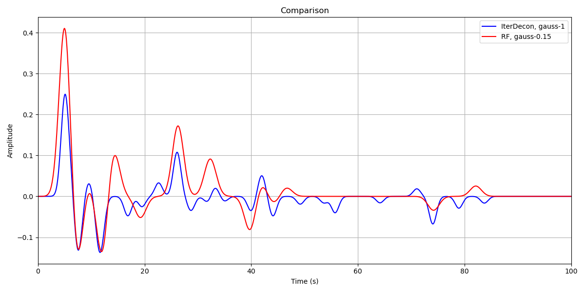
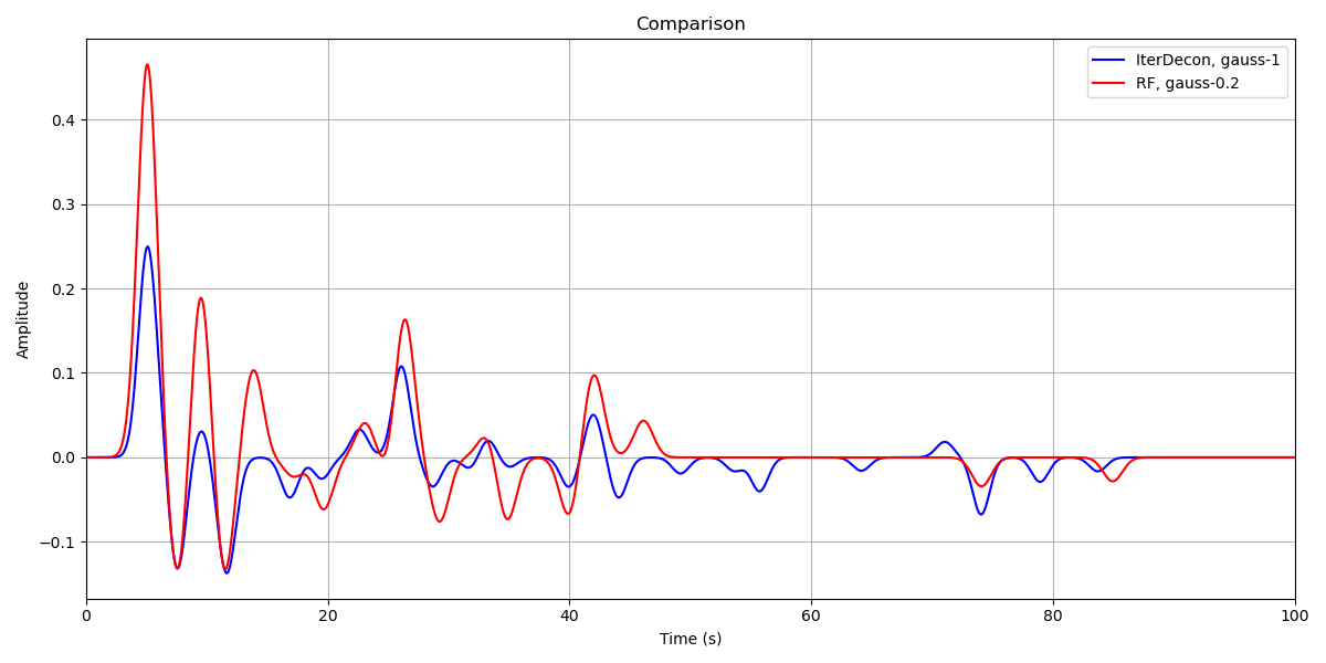
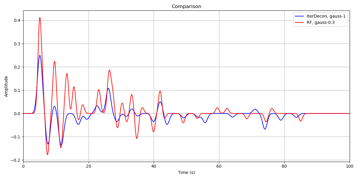
Short answer: The parameters are related like gauss_rf = 0.45 * gauss_id

Long answer:

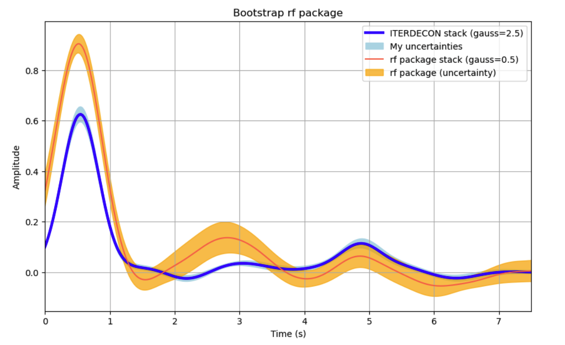
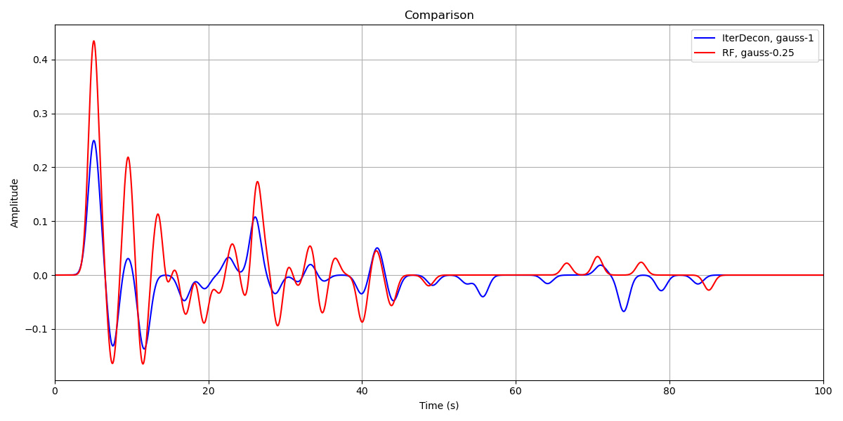
The wiggles of the orange curve (rf) appear to have a longer period than the blue wiggles (id, iterdecon).

In the rf package the gauss parameter is defined as

gauss – Gauss parameter (standard deviation) of the Gaussian Low-pass filter, corresponds to cut-off frequency in Hz for a response value of exp(-0.5)=0.607.

You chose 0.5 for rf’s gauss, that is a 0.5 Hz lowpass → periods will be ~2s or larger → “rf peaks” will be >2s apart, which is what you observe in your plot (fist peak at 0.5s, 2nd at >2.5s).

Looking at the code, the definition of the filter response in frequency domain is

exp(-0.5 * (f/gauss_rf) ** 2)

I do not know the definition of the gauss parameter in iterdecon, but looking at the code of iterdeconvd.f, lines 518-566 the Gaussian filter response should be

exp(-pi**2 * (f/gauss_id) ** 2)

Therefore: gauss_rf = sqrt(2) / pi * gauss_id = 0.45 * gauss_id

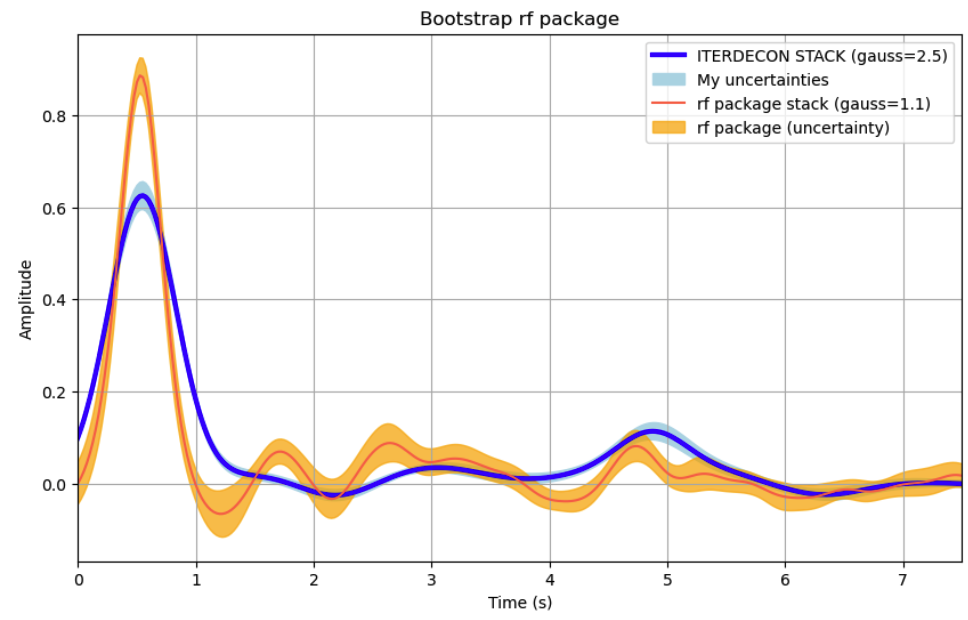
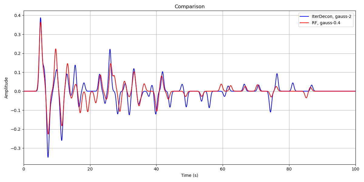
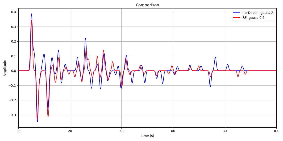
gauss_id 2.5 would be equal to gauss_rf of 1.1. And indeed, higher frequencies are still present for the iterdecon curve, there is a small peak at ~1.5s in the blue curve.

[Ademar]

Thank you so much for your complete response. Here, I uploaded the comparison when the gauss_rf is 1.1 :

I am unsure about what am I doing wrong in my code, so I will show you my goal. Here is the SAC code I am using to compute the RFs:

r *HHZ* *HHR* *HHT*
rtrend
rmean
taper
bandpass corner 0.05 5 npoles 2 passes 2
w V.SAC R.SAC T.SAC
quit
END1

And then run the deconvolution code (ALP is alpha or Gaussian parameter):

saciterd -FN R.SAC -FD V.SAC -N 1000 -ALP 2.5 

The result of this code is the blue RF we saw above. Now, for calculating the orange RF, my jupyter notebook is doing the following:

#lowpass filter first
stream.filter('lowpass', freq=5, corners=2, zerophase=True)

#Then apply a highpass filter
stream.filter('highpass', freq=0.05, corners=2, zerophase=True)

#and now, deconvolution:
rf_iter = stream.copy().rf(deconvolve='iterative', gauss=1.1 ,itmax=1000, minderr=0.001, mute_shift=False, normalize=0).moveout()

What am I doing wrong? Why now that I have the gauss_rf=1.1 and gauss_id=2.5 the traces do not look like having the same pulse width?

I am very grateful for your response. Thanks a lot!

[trichter]

TBH, I do not know why the two rfs look different. At least they show similar features. Could be that the two codes handle the iterative deconvolution slightly differently. @hfmark contributed the iterative deconvolution code to rf, maybe she knows more.

[hfmark]

It’s been a while since I wrote the function so I don’t remember all of what I did to test it, but I think I was mostly checking that it gave similar results to the other decon methods in the package. I’m also not sure why the two look different, to be honest; in theory the method is all the same.

You might want to first check the sac vs obspy filters to make sure they’re doing similar things to your input data. You can also try using the private methods in rf that construct the gaussian filter to take a look at the pulse width you get for a given gauss parameter and see if it matches your expectations. I’ll note that normalization in Ammon’s codes is handled in particular way (the last section of this webpage: "Receiver Function Source Equalization") so perhaps that is part of it?

[Ali_Aslanli]

Hello!

I’ve stumbled upon the same question. It seems to me that the most optimum ratio btw. IterDecon and RF package for the gaussian parameter is in between 4-5 as mentioned by OP.

Another thing that should be taken into account is the moveout correction. The IterDecon originally does not use this correction (as far as I know), so for the comparison it is better not to use it in RF package, otherwise the signals will be out of phase.

Posting some results for the comparison:

[trichter]

Hey!

Thanks for your input. I took another look at the iterdeconvd.f code and confirmed:

gauss_freq_response = exp(-0.5 * (f/gauss_rf) ** 2) = exp(-pi**2 * (f/gauss_id) ** 2)

but there was a serious error after that. As I see now:

gauss_rf = sqrt(0.5) / pi * gauss_id = 0.22 * gauss_id

Voilà!
0.22 resp. the inverse 4.44 are the correct factors, sorry for the confusion.