Array response ( questions)

Hello Martin Gal and the rest of obspy users,

First of all thank you so much for your rapid response.

  1. Comments of the array,

The mean depth value of this deployment is at 4800 m, ant the data I will finally try to handle is going to be treated to avoid “tilt noise” and the microseism noise", so my idea is to reduce the overall noise to a good snr level.

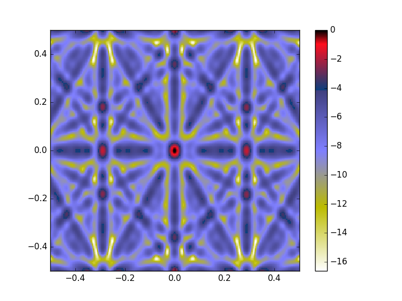
As you told me I’ve been trying to plot my array response by using array_transff_freqslowness(), but something is wrong when i try to draw it.(I ve attach my script). So in your last email did you suggest that I have to plot ( sx,sy) plot and the module(s) versus frecuency right? do you have any example??

  1. Another good question.

there is some way in obspy to make stack, to get a beamforming seismogram ( I mean to, I have the 5 seismograms and I would like to get the coherent sum of that), this is because in the example https://docs.obspy.org/tutorial/code_snippets/beamforming_fk_analysis.html, it show a kind of vespagram more than a beamforming seismogram.

Script

import numpy as np
import matplotlib.pyplot as plt

from obspy.imaging.cm import obspy_sequential
from obspy.signal.array_analysis import array_transff_freqslowness

generate array coordinates

coords = np.array([[-10.373608,35.909685, 0.021], [-10.554655,35.594688, 0.154], [-10.988262,35.595025,0.023],[-10.988500, 36.220166,0.204], [-10.555266,36.220216,0.003]])
#coords /= 1000.

#Slowness units are in s/m ¿this is right)

#frecuency units are in Hz, limit sample frecuency/2

slim= 0.001
sxmin = -slim
sxmax = slim
symin = -slim
symax = slim
sstep = slim / 100.
flim = 25
fstep= flim / 100.
fmax=flim
fmin=0
array_transff_freqslowness(coords, slim, sstep, fmin, fmax, fstep,coordsys=‘lonlat’)
plt.pcolor(np.arange(sxmin, sxmax + sstep * 1.1, sstep) - sstep / 2.,
np.arange(symin, symax + sstep * 1.1, sstep) - sstep / 2.)
plt.colorbar()
plt.clim(vmin=0., vmax=1.)
plt.xlim(sxmin, sxmax)
plt.ylim(symin, symax)
plt.show()

I am very grateful for anyone that could help me, :slight_smile:

Hi Roberto,

The plotting issue is just that you haven’t passed the output of array_transff_freqslowness to pcolor, try the following,

transff=array_transff_freqslowness(coords, slim, sstep, fmin, fmax, fstep,coordsys=‘lonlat’)

plt.pcolormesh(np.arange(sxmin, sxmax + sstep * 1.1, sstep) - sstep / 2.,

np.arange(symin, symax + sstep * 1.1, sstep) - sstep / 2.,

transff)

also pcolormesh is renders faster than pcolor but gives the same result.

best, Dave

Hi Roberto,

please note that there is a long running pull request for a lot more
array analysis stuff open at github:
https://github.com/obspy/obspy/pull/1002

You should definitely have a look if you're doing array analysis.

cheers,
T

Hi Roberto,

With the correction of Dave and a few changed parameters, I get the
enclosed result. The changed code is:

import numpy as np
import matplotlib.pyplot as plt
from obspy.imaging.cm import obspy_sequential
from obspy.signal.array_analysis import array_transff_freqslowness

coords = np.array([[-10.373608,35.909685, 0.021], [-10.554655,35.594688,
0.154], [-10.988262,35.595025,0.023],[-10.988500, 36.220166,0.204],
[-10.555266,36.220216,0.003]])

slim= 0.5
sxmin = -slim
sxmax = slim
symin = -slim
symax = slim
sstep = slim / 100.
fstep= 0.05
fmax=0.3
fmin=0.1
transff=array_transff_freqslowness(coords, slim, sstep, fmin, fmax,
fstep,coordsys='lonlat')
plt.pcolormesh(np.arange(sxmin, sxmax + sstep * 1.1, sstep) - sstep /
2.,
                          np.arange(symin, symax + sstep * 1.1, sstep) -
sstep / 2.,
                          10*np.log10(transff),cmap='gist_stern_r')

plt.colorbar()
plt.xlim(sxmin, sxmax)
plt.ylim(symin, symax)
plt.show()

Slowness is in s/km and frequency is in Hz. Also, I have changed the
output power to decibel with 10*np.log10(), as this should be a
standard. Otherwise you might not see sidelobe contributions at all.

You might want to insert your frequency of interest and see how the
array responds.

To your second question. Generating a coherent sum of the 5 stations is
only to a degree possible. If you are interested in the seismogram of
the strongest source, you can perform a beamforming analysis. With the
estimated slowness and azimuth you can calculate the travel times
between stations and build a coherent stack for the strongest source.
This procedure however does not remove the other signal, but they are
incoherently summed and their contribution will decrease with the
increasing number of stations. Given that you have only 5 stations, the
result might not be the best.

The figure that you refer to as a beamforming vespagram is a simple
power,slowness and azimuth over time analysis. The supplied seismic
traces are split into smaller time samples, and a beamforming analysis
is performed for all of them. Then the parameters for the strongest
source in each time window is plotted in these graphs. It will give you
information on the temporal properties of your seismic trace.

Cheers,
Martin

obspy_mailinglist1.png