Hi all,
ObsPy version: 1.1.1.post0+1050.g345506c439
Python version: 3.7.3
Platform: OsX and Anaconda
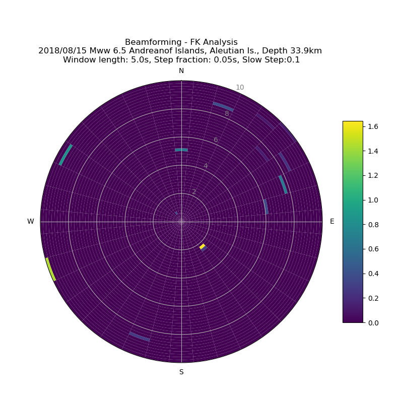
So I’m currently working on some teleseismic events recorded by the Swiss network (as an array). I want to analyze the incoming body and surface waves using vespagrams (time/backazimuth vs. slowness), but there aren’t any related Obspy functions. I tried using the array_processing module and the example here to see if I can get some results that make sense (see the code below). I would expect to see similar results even with slightly different slowness steps, but it gave totally different results.
Then I found this example notebook that has almost all the functions I’m looking for. However, the code is written in old python and obspy version. I tried to rewrite some parts to fit python 3 and my obspy version, but some functions are just no longer present in obspy/somehow present in a different module (e.g. vespagram_baz).
Can someone here who is an expert in these array processing functions point me to the right direction? And will the Obspy Team rewrite and implement these useful functions from the example notebook in Obspy?
Thanks for your help!
Python code:
import obspy
import sys
from obspy.geodetics.base import gps2dist_azimuth  # distance in m, azi and bazi in degree
from obspy.geodetics import kilometers2degrees     # distance in degree
import numpy as np
import matplotlib.pyplot as plt
import string
from obspy.geodetics.flinnengdahl import FlinnEngdahl
from obspy.imaging.cm import obspy_sequential
from obspy.signal.array_analysis import array_processing
from matplotlib.colorbar import ColorbarBase
from matplotlib.colors import Normalize
from obspy.taup import TauPyModel

# Parameters
components_eval = ['HHZ'] # Select components
method = "DLS"
phase_list = ["P"] # Phase list
model = "iasp91" # bg model
# model = "ak135"
model_ev = TauPyModel(model=model)
nthroot = 4 # nth root, 1=linear
scale = 25  # scaling
# f = 0.1   # lowpass/highpass frequency
f1 = 0.3    # freqmin
f2 = 3.0      # freqmax
slow = (-10, 10, 0.1) # Slowness lower bound, upper bound, intervals
static3D = False # static correction
vel_corr = 4.8  # crustal velocity for correction

# Read data and catalog information
event_name = "Alaska_20180815_M6.5"

from obspy.clients.fdsn import Client
starttime = obspy.UTCDateTime("2018-08-15 21:56:56")
endtime   = starttime + 7200

client = Client("ETH")
st = client.get_waveforms("CH", "*", "*", "HHZ", starttime, endtime)
inventory = client.get_stations(network="CH", station="*", channel="HHZ",level="response",
                                starttime=starttime, endtime=endtime)

cat = obspy.read_events("catalog.ml", format="QUAKEML")
ev  = cat[0]
origin    = ev.preferred_origin()
lat_event = origin.latitude
lon_event = origin.longitude
dep_event = origin.depth/1000.
ev_otime = origin.time
time_event_sec = ev_otime.timestamp
year   = ev_otime.year
month  = ev_otime.month
day    = ev_otime.day
hour   = ev_otime.hour
minute = ev_otime.minute
second = float(ev_otime.second) + ev_otime.microsecond / 1E6

if ev.preferred_magnitude().magnitude_type in ["mw", "mww"]:
        mag_type  = ev.preferred_magnitude().magnitude_type
        mag_event = ev.preferred_magnitude().mag
else:
    for _i in ev.magnitudes:
        if _i.magnitude_type in ["Mw", "Mww"]:
            mag_type  = _i.magnitude_type
            mag_event = _i.mag

fe = FlinnEngdahl()
region = fe.get_region(lon_event,lat_event)

# read all the inventories
array_list = []
P_arrival = np.array([])
st1 = obspy.Stream()
for i, tr in enumerate(st):
    pre_filt = [0.001, 0.005, 10, 20]
    tr.remove_response(inventory=inventory, pre_filt=pre_filt, output="DISP", water_level=60, plot=False)

    lat_sta = inventory[0][i].latitude
    lon_sta = inventory[0][i].longitude
    elv_sta = inventory[0][i].elevation /1000. # in km
    dist, azi, bazi = gps2dist_azimuth(lat_event, lon_event, lat_sta, lon_sta)
    dist_deg        = kilometers2degrees(dist/1000.) # in km
    tr.stats["coordinates"] = {} # add the coordinates to your dictionary, needed for the section plot
    tr.stats["coordinates"]["latitude"]  = lat_sta
    tr.stats["coordinates"]["longitude"] = lon_sta
    tr.stats["coordinates"]["elevation"] = elv_sta

    st1 += tr
    array_list.append([tr.stats.network,tr.stats.station,tr.stats.location,lat_sta,lon_sta,bazi,dist_deg,elv_sta])

    arr = model_ev.get_ray_paths(source_depth_in_km=dep_event, distance_in_degree=dist_deg, phase_list=["P"])
    P_arrival = np.append(P_arrival, arr[0].time)

# Read sorted seismograms and inventories
if len(st1) == 0 or len(inventory) == 0:
    sys.exit("Station list is empty! Please check!")

print("Number of stations used:", len(st1))

# filter the data
st_new = st1.copy()
st_new.resample(10) # downsample to 10 Hz
st_test = st_new.copy()

# Filtered
st_new.taper(0.02, 'cosine')
st_new.detrend("demean")
st_new.detrend('linear')
st_new.filter("bandpass", freqmin=f1, freqmax=f2, corners=2, zerophase=True)
# st.filter("lowpass", freq=f, corners=2, zerophase=False)

# detrend after filtering
st_new.detrend('linear')
# choose the maximun and minimum of the starting times
starttime = max([tr.stats.starttime for tr in st_new])
endtime   = min([tr.stats.endtime for tr in st_new])
st_new.trim(starttime, endtime, pad=True, fill_value=0)

# Non-filtered
# st_test.taper(0.02, 'cosine')
# st_test.detrend("demean")
# st_test.detrend('linear')
# starttime2 = max([tr.stats.starttime for tr in st_test])
# endtime2   = min([tr.stats.endtime for tr in st_test])
# st_test.trim(starttime2, endtime2, pad=True, fill_value=0)


# Execute array_processing
kwargs = dict(
    # slowness grid: X min, X max, Y min, Y max, Slow Step
    sll_x=-10.0, slm_x=10.0, sll_y=-10.0, slm_y=10.0, sl_s=0.1,
    # sliding window properties
    win_len=5., win_frac=0.05,
    # frequency properties
    frqlow=f1, frqhigh=f2, prewhiten=0,
    # restrict output
    semb_thres=-1e9, vel_thres=-1e9,
    stime=starttime+int(min(P_arrival))-5,
    etime=starttime+int(max(P_arrival))+5
)

out = array_processing(st_new, **kwargs)
# out = array_processing(st_test, **kwargs)

# Plot
cmap = obspy_sequential

# make output human readable, adjust backazimuth to values between 0 and 360
t, rel_power, abs_power, baz, slow = out.T
baz[baz < 0.0] += 360

# choose number of fractions in plot (desirably 360 degree/N is an integer!)
N  = 36
N2 = 50
abins = np.arange(N + 1) * 360. / N
sbins = np.linspace(0, 10, N2 + 1)

# sum rel power in bins given by abins and sbins
hist, baz_edges, sl_edges = \
    np.histogram2d(baz, slow, bins=[abins, sbins], weights=rel_power)

# transform to radian
baz_edges = np.radians(baz_edges)

# add polar and colorbar axes
fig = plt.figure(figsize=(8, 8))
cax = fig.add_axes([0.85, 0.2, 0.05, 0.5])
ax = fig.add_axes([0.10, 0.1, 0.70, 0.7], polar=True)
ax.set_theta_direction(-1)
ax.set_theta_zero_location("N")

dh = abs(sl_edges[1] - sl_edges[0])
dw = abs(baz_edges[1] - baz_edges[0])

# circle through backazimuth
for i, row in enumerate(hist):
    bars = ax.bar(x=(i * dw) * np.ones(N2),
                  height=dh * np.ones(N2),
                  width=dw, bottom=dh * np.arange(N2),
                  color=cmap(row / hist.max()))

ax.set_xticks(np.linspace(0, 2 * np.pi, 4, endpoint=False))
ax.set_xticklabels(['N', 'E', 'S', 'W'])

# set slowness limits
ax.set_ylim(0, 10)
[i.set_color('grey') for i in ax.get_yticklabels()]
ColorbarBase(cax, cmap=cmap,
              norm=Normalize(vmin=hist.min(), vmax=hist.max()))

plt.title('Beamforming - FK Analysis\n'+"%04d"% year+'/'+
          "%02d"% month +'/'+"%02d"% day+' '+mag_type.capitalize()+' '+
          "%.1f"% mag_event+' '+string.capwords(region) +', Depth '+ "%.1f"% dep_event+'km \n' +
          "Window length: "+str(kwargs["win_len"])+"s, Step fraction: "+str(kwargs["win_frac"])+"s, Slow Step:" +str(kwargs["sl_s"]))

plt.show()