# How to import my own SAC data and calculate SRF
**URL:** https://discourse.obspy.org/t/how-to-import-my-own-sac-data-and-calculate-srf/1229
**Category:** Related: rf
**Created:** [May 4, 2021, 1:39pm UTC](https://discourse.obspy.org/t/how-to-import-my-own-sac-data-and-calculate-srf/1229 "2021-05-04T13:39:00Z")
**Posts on this page:** 12
**Page:** 1
### Author:  [@geoAP90](https://discourse.obspy.org/u/geoAP90)
#### Post date: [May 4, 2021, 1:39pm UTC](https://discourse.obspy.org/t/how-to-import-my-own-sac-data-and-calculate-srf/1229/1 "2021-05-04T13:39:00Z")
1. I need to understand how should I import my own data and make the figures
2. I have a set of calculated and selected P-RF. Can I import the .eqr files and just plot the figures using RF software?
---
### Author:  [@trichter](https://discourse.obspy.org/u/trichter)
#### Post date: [May 4, 2021, 4:57pm UTC](https://discourse.obspy.org/t/how-to-import-my-own-sac-data-and-calculate-srf/1229/2 "2021-05-04T16:57:01Z")
1. Please have look here:
> [@RF, reading SAC downloaded via SOD](https://discourse.obspy.org/t/rf-reading-sac-downloaded-via-sod/1138):
>
> Fairly new to ObsPy; sorry a likely naive question, I have SAC files (network=US; station name=GLMI; components; BH1, BH2, BHZ) downloaded using SOD and want to calculate a receiver function using RF. Following the manual, I succeed to read: from rf import read\_rf, rfstats, RFStream data = read\_rf(‘US.GLMI.00.BH?.sac’) stream = RFStream() print('aa ', data[0].stats.sac.kstnm) returns: aa GLMI but the command: stats = rfstats(station=station, event=event, phase=‘P’, dist\_range=(30,90)) r…
1. Probably not, rf only supports waveforms which can be read by ObsPy.
---
### Author:  [@geoAP90](https://discourse.obspy.org/u/geoAP90)
#### Post date: [May 14, 2021, 7:20am UTC](https://discourse.obspy.org/t/how-to-import-my-own-sac-data-and-calculate-srf/1229/3 "2021-05-14T07:20:27Z")
Hey this is me again. I am trying to calculate P-RF of my selected dataset. I could run the python codes given in notebook 1 and got my results but when I am trying to run the iterative deconvolution , I am not getting the desired result.
I have used the following codes
Step 1.
import matplotlib.pyplot as plt
from rf import read\_rf, rfstats
stream = read\_rf(‘/home/arpita/Documents/LADAKH/select/DRBK\*’, debug\_headers=True)
print(stream)
print(‘\nStats:\n’, stream[0].stats)
stream[:3].plot()
step 2
rfstats(stream)
stream.filter(‘bandpass’, freqmin=0.4, freqmax=1)
stream.trim2(5, 95, ‘starttime’)
print(stream)
stream[:3].plot(type=‘relative’, reftime=stream[0].stats.onset)
step3
stream.rf()
stream.moveout()
stream.trim2(-5, 22, ‘onset’)
print(stream)
stream.select(component=‘L’).plot\_rf()
stream.select(component=‘Q’).plot\_rf()
plt.show()
step 4
import matplotlib.pyplot as plt
from rf import read\_rf, rfstats
stream = read\_rf(‘/home/arpita/Documents/LADAKH/select/DRBK\*’, debug\_headers=True)
rfstats(stream)
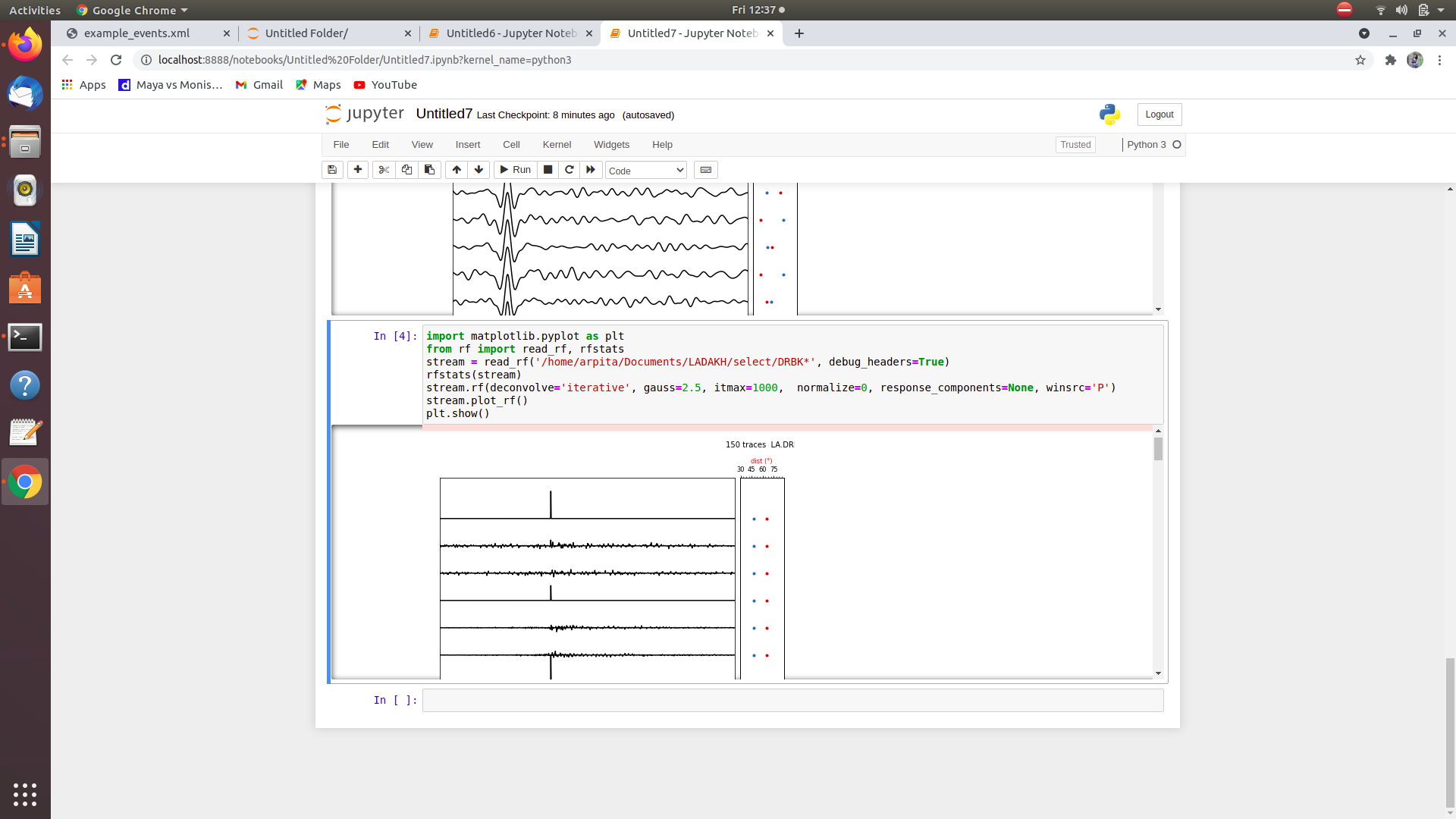
stream.rf(deconvolve=‘iterative’, gauss=2.5, itmax=1000, normalize=0, response\_components=None, winsrc=‘P’)
stream.plot\_rf()
plt.show()
I am attaching the resultant rf that I am getting which is not matching with my desired one. P.S I have already calculated the P-RF of this set of SAC files using Liggorias iterative deconvolution and that is how I know how the final figure should look like.
Can you please assist me here to understand where I am doing the steps wrong to get my P-RF?
---
### Author:  [@hfmark](https://discourse.obspy.org/u/hfmark)
#### Post date: [May 14, 2021, 1:45pm UTC](https://discourse.obspy.org/t/how-to-import-my-own-sac-data-and-calculate-srf/1229/4 "2021-05-14T13:45:49Z")
Hi - have you tried filtering your data after you re-import it in step 4? Unless the data you’re reading in have already been filtered elsewhere that might be a good place to start for figuring this out.
---
### Author:  [@geoAP90](https://discourse.obspy.org/u/geoAP90)
#### Post date: [May 15, 2021, 5:38am UTC](https://discourse.obspy.org/t/how-to-import-my-own-sac-data-and-calculate-srf/1229/5 "2021-05-15T05:38:41Z")
import matplotlib.pyplot as plt
from rf import read\_rf, rfstats
stream = read\_rf(‘/home/arpita/Documents/LADAKH/select/DRBK\*’, debug\_headers=True)
rfstats(stream)
stream.filter(‘bandpass’, freqmin=0.4, freqmax=1)
stream.rf(deconvolve=‘iterative’, gauss=2.5, itmax=1000, normalize=0, response\_components=None, winsrc=‘P’)
stream.plot\_rf()
plt.show()
So I added the 5th line for filtering the data but still found no much change in the outcome.
---
### Author:  [@hfmark](https://discourse.obspy.org/u/hfmark)
#### Post date: [May 16, 2021, 1:11am UTC](https://discourse.obspy.org/t/how-to-import-my-own-sac-data-and-calculate-srf/1229/6 "2021-05-16T01:11:04Z")
I’m not familiar with Liggorria’s code so it’s hard to tell what might cause you to get different results, but you might check how the gaussian parameter is defined in that code versus this one. The value you input (2.5) might not mean exactly the same thing in the calculation here as it does in the other code. Also, depending on the length of the traces you’re using, it’s possible that trimming them before the deconvolution would help, though that effect is probably small since you’ve set the number of iterations fairly high at 1000.
---
### Author:  [@geoAP90](https://discourse.obspy.org/u/geoAP90)
#### Post date: [May 16, 2021, 3:56pm UTC](https://discourse.obspy.org/t/how-to-import-my-own-sac-data-and-calculate-srf/1229/7 "2021-05-16T15:56:55Z")
Thanks for your response. I have tried to play with the number of iterations and gaussian value also I have trimmed the data but still not finding much change in the figure. All I am trying to get is the figures that are displayed in notebook 2 example but with my own sac data. I can obtain the same images given in notebook 1 using the commands. Can you please guide me to understand how should I change the commands given in notebook 2 to obtain results with my own sac files?
---
### Author:  [@trichter](https://discourse.obspy.org/u/trichter)
#### Post date: [May 17, 2021, 9:47am UTC](https://discourse.obspy.org/t/how-to-import-my-own-sac-data-and-calculate-srf/1229/8 "2021-05-17T09:47:13Z")
Indeed, those receiver functions look messy, with some peaks on the source component going up and some going down. In step 3 the rfs look as expected? Can you try to feed only 3 traces from one event to the rf method? By the way, you can leave away the kwargs normalize, response\_components, winsrc which you only set to the default values.
---
### Author:  [@geoAP90](https://discourse.obspy.org/u/geoAP90)
#### Post date: [May 19, 2021, 8:48am UTC](https://discourse.obspy.org/t/how-to-import-my-own-sac-data-and-calculate-srf/1229/9 "2021-05-19T08:48:22Z")
hello trichter . Finally I can plot my own sac files in RF with a slight change in some codes .
I can plot the time domain waterlevel deconvolution using this . But as I am changing the ‘time’ parameter into ‘freq’ ‘iter’ or ‘multi’ some error messages are appearing. How should I make it flexible to calculate both iterative and waterlevel deconvolution?
if calculcate\_RF==“PRF”:
RFstream.rf(deconvolve=‘time’,rotate=‘NE-\>RT’,solve\_toeplitz=‘scipy’)
---
### Author:  [@trichter](https://discourse.obspy.org/u/trichter)
#### Post date: [May 19, 2021, 1:51pm UTC](https://discourse.obspy.org/t/how-to-import-my-own-sac-data-and-calculate-srf/1229/10 "2021-05-19T13:51:53Z")
It is difficult to help you without more information. Can you provide a short self-contained example?
---
### Author:  [@geoAP90](https://discourse.obspy.org/u/geoAP90)
#### Post date: [May 20, 2021, 5:57am UTC](https://discourse.obspy.org/t/how-to-import-my-own-sac-data-and-calculate-srf/1229/11 "2021-05-20T05:57:53Z")
Yes I can send a sample data. Should I mail it to you?
---
### Author:  [@trichter](https://discourse.obspy.org/u/trichter)
#### Post date: [May 20, 2021, 5:45pm UTC](https://discourse.obspy.org/t/how-to-import-my-own-sac-data-and-calculate-srf/1229/12 "2021-05-20T17:45:55Z")
Thanks for the waveforms, but I can only only iterate:
> It is difficult to help you without more information.
For example, can you specify which error messages are appearing.